Introduction to EXPLAIN
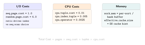
The EXPLAIN output reports five numbers per node: startup cost, total cost, estimated rows, row width, and — with ANALYZE — actual timing. This module teaches you to read those numbers and locate the bottleneck node.
Book reference: Chapter 9 — Indexing Strategy
Free preview: Reading EXPLAIN
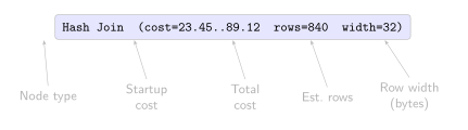
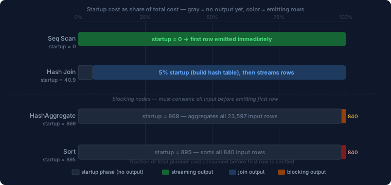
-- startup cost = work before the first row
-- total cost   = work to return all rows
-- High startup signals sorting or hashing.
explain
select d.surname,
       sum(res.points) as career_points
  from f1db.drivers  d
  join f1db.results res
    on res.driverid = d.driverid
 group by d.driverid, d.surname
 order by career_points desc
 limit 10;
EXPLAIN plan for the top 10 drivers ranked by total career points across all seasons.
EXPLAIN ANALYZE in Practice
EXPLAIN ANALYZE runs the query and adds actual rows, actual time, and loop counts. The gap between estimated and actual rows is the key signal — it tells you where the planner's model breaks down.
Book reference: Chapter 9 — Indexing Strategy
Free preview: Reading EXPLAIN
-- rows=N (estimate) vs actual rows=N
-- A large gap means stale statistics or
-- correlated predicates.
explain (analyze, buffers)
select r.year,
       r.round,
       r.name
  from f1db.races r
 where r.year  = 2017
   and r.round <= 10;
EXPLAIN ANALYZE output for 2017 season races filtered to the first ten rounds.
Plan Node Types: Scans and Joins
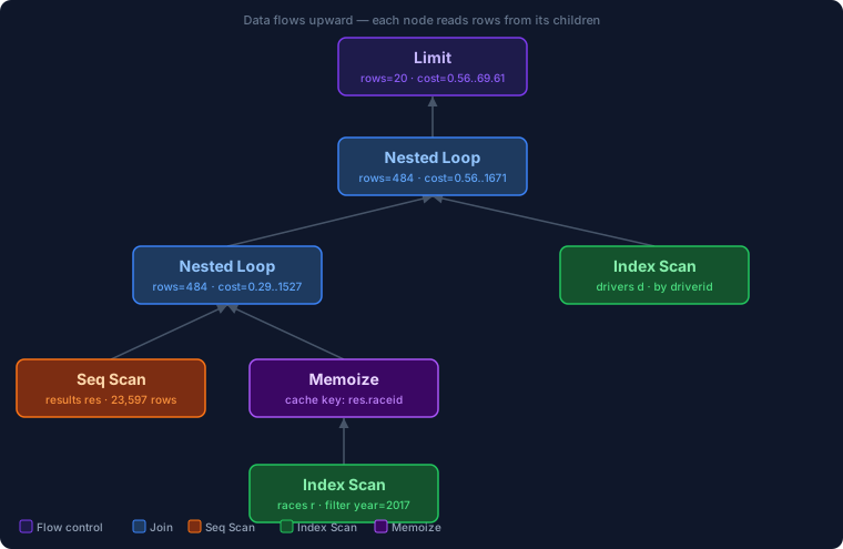
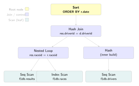
The executor processes a tree of plan nodes, each producing tuples for its parent until the root node drives the whole thing. This module covers the scan and join nodes that fetch and combine rows.
Book reference: Chapter 9 — Indexing Strategy
Free preview: Reading EXPLAIN
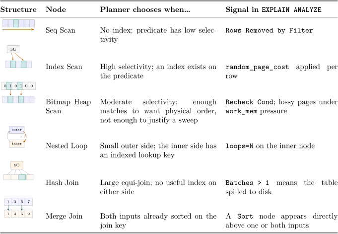
-- Hash Join: build a hash table from the
-- smaller relation, probe with each row
-- from the larger. Build cost = startup.
explain (analyze, buffers)
select d.nationality,
       count(distinct d.driverid)   as drivers,
       count(*) filter(
         where res.positionorder=1) as wins
  from f1db.results res
  join f1db.drivers d
    on d.driverid = res.driverid
  join f1db.races   r
    on r.raceid   = res.raceid
 where r.year = 2017
 group by d.nationality
 order by wins desc;
EXPLAIN ANALYZE for driver and win counts by nationality in the 2017 season.
Plan Node Types: Aggregation and Parallel Execution
After scans and joins fetch and combine rows, this module covers what happens next: grouping, ordering, combining results from sub-plans, and running parts of the plan across multiple workers.
Book reference: Chapter 9 — Indexing Strategy
Free preview: Reading EXPLAIN
-- Every window query needs a Sort node
-- to feed the WindowAgg node.
-- Incremental Sort can reduce this cost.
explain (analyze, buffers)
select r.year,
       d.surname,
       sum(res.points) over(
         partition by r.year, d.driverid
         order by r.date
         rows between unbounded preceding
                  and current row
       ) as running_points
  from f1db.results res
  join f1db.races   r
    on r.raceid   = res.raceid
  join f1db.drivers d
    on d.driverid = res.driverid
 where r.year = 2017
   and d.driverid in (1, 8, 20)
 order by r.date, d.surname;
Running cumulative points per driver by race date for three drivers in the 2017 season.
Statistics and the Planner
Every `rows=` figure in a plan is an estimate computed from statistics ANALYZE collected — not a measurement. This module traces row estimates back to the MCV list and histogram that produced them.
Book reference: Chapter 9 — Indexing Strategy
Free preview: Reading EXPLAIN
-- geoname.class and .feature are strongly
-- correlated: 'PPL' always implies class 'P'.
-- The planner multiplies selectivities as
-- if they were independent and lands far
-- below the actual row count.
explain (analyze, buffers)
select name, population
  from geoname.geoname
 where class   = 'P'
   and feature = 'PPL';
EXPLAIN ANALYZE plan for geoname rows matching both class 'P' and feature 'PPL'.
Detecting Performance Issues
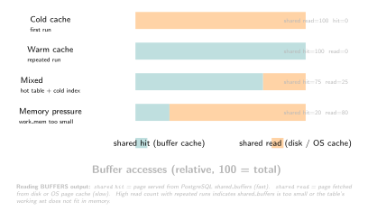
Batches > 1 on a HashJoin means the hash table spilled to disk. Sort Method: external merge means the sort did too. Rows × loops mismatches point to bad estimates compounding through the tree.
Book reference: Chapter 9 — Indexing Strategy
Free preview: Reading EXPLAIN
-- Two correlated predicates: positionorder=1
-- and points > 20 are not independent.
-- The planner multiplies their selectivities
-- and underestimates the actual row count.
explain (analyze, buffers)
select res.raceid,
       res.driverid,
       res.positionorder,
       res.points
  from f1db.results res
 where res.positionorder = 1
   and res.points > 20;
Results rows where finishing position is first and points scored exceed 20.
Building a Diagnostic Workflow
pg_stat_activity for live query monitoring, lock monitoring with pg_locks, and CREATE STATISTICS for correlated columns. How to triage a slow-query incident without disturbing production traffic.
Book reference: Chapter 9 — Indexing Strategy
Free preview: Reading EXPLAIN
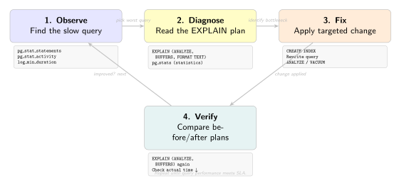
-- Step 1: capture the default plan and cost.
-- Step 2: disable one node type to force an
-- alternative, then compare actual time.
explain (analyze, buffers)
select d.surname,
       sum(res.points) as points
  from f1db.results res
  join f1db.drivers d
    on d.driverid = res.driverid
 group by d.driverid, d.surname
 order by points desc
 limit 10;

-- Then compare:
-- set enable_hashjoin = off;
-- ...same query...
-- reset enable_hashjoin;
Total career points per driver ranked descending, limited to the top 10.
Observability and Performance Strategy
VACUUM signals in EXPLAIN output, autovacuum tuning, and pg_stat_user_tables for table-level health. Connecting plan-level observation to database-wide performance management.
Book reference: Chapter 9 — Indexing Strategy
Free preview: Reading EXPLAIN
-- chinook declares foreign keys; f1db does not.
-- Declared FKs give the planner join-elimination
-- opportunities it cannot use without them.
explain (analyze, buffers)
select ar.name                    as artist,
       count(distinct al.album_id) as albums,
       count(t.track_id)           as tracks,
       round(
         sum(t.milliseconds)
           / 60000.0::numeric, 1
       )                           as total_minutes
  from chinook.artist ar
  join chinook.album  al
    on al.artist_id = ar.artist_id
  join chinook.track  t
    on t.album_id   = al.album_id
 group by ar.artist_id, ar.name
 order by total_minutes desc
 limit 15;
Album count, track count, and total playing time per chinook artist, top 15 by runtime.