JOIN Output Cardinality: Why Your Row Counts Surprise You
A JOIN does not just combine tables — it multiplies rows. One-to-many joins inflate counts silently, and aggregate queries over joined data produce wrong results unless you account for it.
Here is a question that trips up developers at every level: how many races has
Ferrari entered in Formula One? The constructors table has one row per team.
The results table has one row per driver per race. A naive count after joining
the two gives the wrong answer:
select c.name                    as constructor,
       count(*)                  as result_rows
  from f1db.constructors c
  join f1db.results res on res.constructorid = c.constructorid
 group by c.constructorid, c.name
 order by result_rows desc
 limit 5;
 constructor │ result_rows
═════════════╪═════════════
 Ferrari     │        2130
 McLaren     │        1615
 Williams    │        1369
 Tyrrell     │         881
 Team Lotus  │         871
(5 rows)
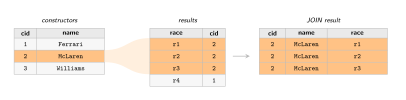
This counts result rows, not distinct races. Ferrari typically enters two cars per race, so the count is roughly twice the number of races entered. For a team with three cars in some eras, the inflation is worse.
This is called join amplification: a one-to-many join multiplies the rows on the “one” side by the number of matching rows on the “many” side. The query compiles and returns results. The results are wrong.
The fix: count what you actually mean
If you want distinct races, count distinct race IDs:
select c.name                        as constructor,
       count(distinct res.raceid)    as races_entered,
       count(distinct res.driverid)  as distinct_drivers
  from f1db.constructors c
  join f1db.results res on res.constructorid = c.constructorid
 group by c.constructorid, c.name
 order by races_entered desc
 limit 5;
 constructor │ races_entered │ distinct_drivers
═════════════╪═══════════════╪══════════════════
 Ferrari     │           946 │               95
 McLaren     │           775 │               51
 Williams    │           689 │               53
 Tyrrell     │           433 │               47
 Team Lotus  │           395 │               61
(5 rows)
COUNT(DISTINCT res.raceid) counts each race once regardless of how many
result rows belong to it. The same query now correctly answers two questions
at once: how many races and how many different drivers.
The mental model
When you write A JOIN B ON A.id = B.a_id and there are multiple B rows
per A row, the output has one row per (A, B) pair — not one row per A.
This is correct and expected behaviour. The issue is not the JOIN; it is
failing to account for it in the aggregate.
Before aggregating over a join, ask: for each group, what is the right
denominator? COUNT(*) counts pairs. COUNT(DISTINCT col) counts unique
values in one of the joined tables. Often the right answer is to aggregate
before joining, not after.
Aggregate before joining
The problem compounds when two “many” tables are joined at once.
constructorresults records the points each constructor scored in each race —
one row per (constructor, race). results records every driver entry —
multiple rows per (constructor, race). Joining both before aggregating
silently multiplies each points row by the number of driver entries that race:
select c.name,
       sum(cr.points) as season_points,
       count(*)       as row_count
  from f1db.constructors        c
  join f1db.constructorresults cr using (constructorid)
  join f1db.results            res using (constructorid, raceid)
  join f1db.races                r using (raceid)
 where r.year = 2016
 group by c.constructorid, c.name
 order by season_points desc
 limit 5;
    name     │ season_points │ row_count
═════════════╪═══════════════╪═══════════
 Mercedes    │          1530 │        42
 Red Bull    │           936 │        42
 Ferrari     │           796 │        42
 Force India │           346 │        42
 Williams    │           276 │        42
(5 rows)
Mercedes’ actual 2016 constructor championship total is 765 points. The join
doubles it: 2016 had 21 races, each constructor entered 2 drivers, so each
constructorresults row matches 2 results rows and is summed twice. The
42 in row_count is the tell — 21 races × 2 drivers. There is no DISTINCT
fix for SUM. The right approach collapses each “many” side to one row per
constructor before joining:
with season_points as (
  select cr.constructorid,
         r.year,
         sum(cr.points) as season_points
    from f1db.constructorresults cr
    join f1db.races r using (raceid)
   group by cr.constructorid, r.year
),
entries as (
  select res.constructorid,
         r.year,
         count(*) as driver_entries
    from f1db.results res
    join f1db.races r using (raceid)
   group by res.constructorid, r.year
)
select c.name,
       sp.season_points,
       e.driver_entries
  from f1db.constructors c
  join season_points sp using (constructorid)
  join entries        e using (constructorid, year)
 where sp.year = 2016
 order by sp.season_points desc
 limit 5;
    name     │ season_points │ driver_entries
═════════════╪═══════════════╪════════════════
 Mercedes    │           765 │             42
 Red Bull    │           468 │             42
 Ferrari     │           398 │             42
 Force India │           173 │             42
 Williams    │           138 │             42
(5 rows)
Each CTE produces one row per (constructor, year) before any join happens.
The year filter is written once in the outer WHERE — PostgreSQL pushes it
into both CTEs automatically. EXPLAIN makes that visible:
EXPLAIN
with season_points as ( ... ),
     entries       as ( ... )
select ...
 where sp.year = 2016 ...;
 Limit
   -> Sort  (Sort Key: sp.season_points DESC)
       -> Hash Join  (Hash Cond: c.constructorid = e.constructorid)
           -> Hash Join  (Hash Cond: c.constructorid = sp.constructorid)
               -> Seq Scan on constructors c
               -> Hash
                   -> Subquery Scan on sp
                       -> HashAggregate  (Group Key: cr.constructorid)
                           -> Hash Join  (Hash Cond: cr.raceid = r.raceid)
                               -> Seq Scan on constructorresults cr
                               -> Hash
                                   -> Seq Scan on races r
                                         Filter: (year = 2016)   ← pushed down
           -> Hash
               -> Subquery Scan on e
                   -> HashAggregate  (Group Key: res.constructorid)
                       -> Hash Join  (Hash Cond: res.raceid = r_1.raceid)
                           -> Seq Scan on results res
                           -> Hash
                               -> Seq Scan on races r_1
                                     Filter: (year = 2016)   ← pushed down
Filter: (year = 2016) appears inside the races scan in both CTE branches,
not as a post-aggregation filter on the outer result. Since PostgreSQL 12,
non-materialized CTEs are inlined by default and the planner can push
predicates through them. The year column also disappears from the group key
(Group Key: cr.constructorid, not cr.constructorid, r.year) — once the
filter pins year to a constant, grouping by it adds no further distinction.