Reading EXPLAIN

EXPLAIN reveals the plan PostgreSQL chose without running the query. Reading cost, row estimates, and node type fluently is the starting point for all query analysis.

Run it yourself — all queries on this page use the f1db dataset, pre-loaded in the free TAOP lab. Start a session with psql taop and follow along. No setup beyond Docker.

EXPLAIN tells you the plan PostgreSQL chose without executing the query. No rows are produced, no data is changed — the output is the planner’s internal decision written out as text. Learning to read it fluently is the foundation of all performance work.

The simplest plan

The most basic form: wrap any query in EXPLAIN:

explain
select count(*)
  from f1db.results;

                                           QUERY PLAN
══════════════════════════════════════════════════════════════════════════════════════════
 Aggregate  (cost=681.24..681.25 rows=1 width=8)
   ->  Index Only Scan using idx_49569_primary on results  (cost=0.29..622.24 rows=23597 width=0)
(2 rows)

Two nodes. The indentation shows the tree: Index Only Scan feeds rows upward into Aggregate. Each node shows cost=startup..total rows=N width=W:

startup cost — work done before the first row appears (here 0.29 for the index scan, 681.24 for the aggregate that must process everything before it can emit the count)
total cost — estimated total work to produce all rows
rows — estimated number of rows this node will emit
width — average row width in bytes (0 here because count(*) touches no actual columns)

Costs are in arbitrary planner units — what matters is relative comparison between nodes and between two versions of the same query.

Plan trees: reading indentation

A three-table join produces a tree. Indentation shows parent-child structure; data flows upward toward the root:

explain
select d.surname, r.name, res.points
  from f1db.drivers  d
  join f1db.results res on res.driverid = d.driverid
  join f1db.races    r  on r.raceid    = res.raceid
 where r.year = 2017
 limit 20;

 Limit  (cost=0.56..69.61 rows=20 width=34)
   ->  Nested Loop  (cost=0.56..1671.61 rows=484 width=34)
         ->  Nested Loop  (cost=0.29..1527.85 rows=484 width=35)
               ->  Seq Scan on results res  (cost=0.00..647.97 rows=23597 width=24)
               ->  Memoize  (cost=0.29..0.31 rows=1 width=27)
                     Cache Key: res.raceid
                     ->  Index Scan using idx_49556_primary on races r
                           Index Cond: (raceid = res.raceid)
                           Filter: (year = 2017)
         ->  Index Scan using idx_49514_primary on drivers d
               Index Cond: (driverid = res.driverid)

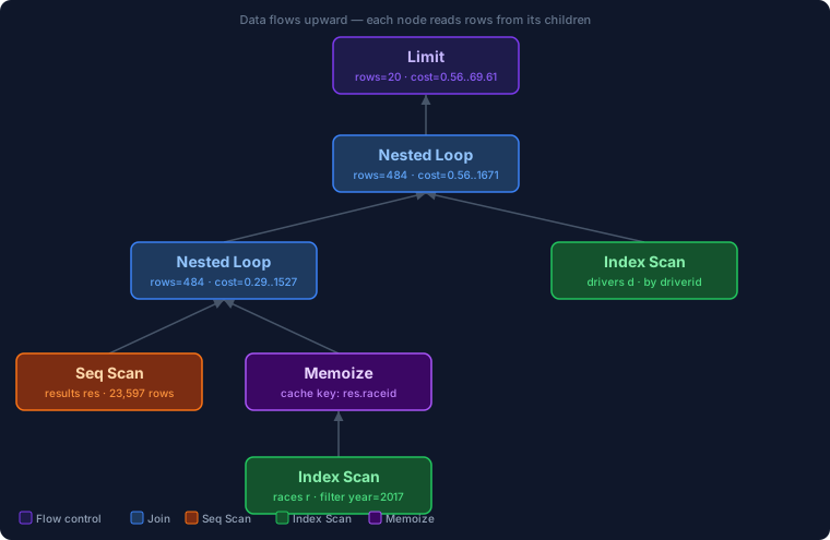
Reading from the leaves upward: results is scanned sequentially, then for each row the Memoize node looks up the matching races row (caching repeated lookups by raceid). Those two streams merge in the inner Nested Loop, then each combined row triggers an index lookup on drivers. The outer Limit stops the outer Nested Loop after 20 rows.

Plan tree for the 3-table join: Limit → Nested Loop → (Nested Loop, Index Scan drivers) → (Seq Scan results, Memoize → Index Scan races)

Startup cost vs total cost

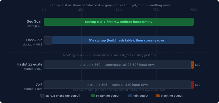
The gap between startup and total cost reveals the node’s behavior:

explain
select d.surname,
       sum(res.points) as career_points
  from f1db.drivers  d
  join f1db.results res on res.driverid = d.driverid
 group by d.driverid, d.surname
 order by career_points desc
 limit 10;

 Limit  (cost=895.66..895.69 rows=10 width=23)
   ->  Sort  (cost=895.66..897.76 rows=840 width=23)
         Sort Key: (sum(res.points)) DESC
         ->  HashAggregate  (cost=869.11..877.51 rows=840 width=23)
               Group Key: d.driverid
               ->  Hash Join  (cost=40.90..751.12 rows=23597 width=23)
                     ->  Seq Scan on results res  (cost=0.00..647.97 rows=23597 width=16)
                     ->  Hash  (cost=30.40..30.40 rows=840 width=15)
                           ->  Seq Scan on drivers d

Sort (cost=895.66..897.76): startup cost 895 means the Sort must consume all 840 input rows before it can return row one — it materializes everything first. A streaming node like Seq Scan (cost=0.00..) has zero startup: it returns the first row immediately.

High startup cost signals: Sort, Hash (build phase), HashAggregate, and CTEs marked MATERIALIZED. These nodes produce no output until they have consumed all input. Everything with cost=0.00..N streams row-at-a-time.

Startup cost as share of total cost: Seq Scan and Hash Join start emitting rows almost immediately; HashAggregate and Sort spend 99%+ of their cost in the startup phase before a single row appears

Seq Scan and the Filter signal

The most important warning in a EXPLAIN output is a Filter on a Seq Scan that removes many rows. This query on all results:

explain
select *
  from f1db.results
 where points >= 0;

 Seq Scan on results  (cost=0.00..706.96 rows=23597 width=138)
   Filter: (points >= '0'::double precision)

All 23,597 rows match, so a Seq Scan is correct here — no index would help. Compare this to EXPLAIN ANALYZE output with Rows Removed by Filter: 22627: that figure tells you 22,627 rows were fetched and discarded. A large removal ratio on a Seq Scan is the clearest signal that an index on the filtered column might cut that work dramatically.

EXPLAIN ANALYZE: seeing what actually ran

Add ANALYZE to execute the query and measure each node:

explain (analyze, format text)
select d.surname, r.name, res.points
  from f1db.drivers  d
  join f1db.results res on res.driverid = d.driverid
  join f1db.races    r  on r.raceid    = res.raceid
 where r.year = 2017
   and res.positionorder = 1
 order by r.date;

 Sort  (cost=754.48..754.53 rows=20) (actual time=1.946..1.948 rows=11 loops=1)
   Sort Method: quicksort  Memory: 25kB
   ->  Nested Loop  (cost=36.73..754.05 rows=20) (actual time=1.897..1.931 rows=11 loops=1)
         ->  Hash Join  (cost=36.45..745.97 rows=20) (actual time=1.881..1.907 rows=11 loops=1)
               Hash Cond: (res.raceid = r.raceid)
               ->  Seq Scan on results res  (cost=0.00..706.96 rows=970) (actual time=0.009..1.750 rows=970 loops=1)
                     Filter: (positionorder = 1)
                     Rows Removed by Filter: 22627
               ->  Hash  (cost=36.20..36.20 rows=20) (actual time=0.091..0.092 rows=20 loops=1)
                     ->  Seq Scan on races r  (cost=0.00..36.20 rows=20) (actual time=0.070..0.084 rows=20 loops=1)
                           Filter: (year = 2017)
                           Rows Removed by Filter: 956
         ->  Index Scan using idx_49514_primary on drivers d (actual time=0.002..0.002 rows=1 loops=11)
               Index Cond: (driverid = res.driverid)
 Planning Time: 0.642 ms
 Execution Time: 2.019 ms

Each node now shows actual time=start..end rows=actual loops=N. The planner estimated 970 rows for positionorder = 1; the actual was also 970 — a good estimate. The loops=11 on the Index Scan on drivers means that node ran 11 times (once per matching result row); times and rows shown are per-loop averages.

One safety rule: EXPLAIN ANALYZE executes the statement. On a SELECT this is safe. On an UPDATE, DELETE, or INSERT, the rows really change. Wrap data-modifying statements in a transaction you roll back:

begin;
explain (analyze, buffers)
  update f1db.results set points = points where resultid = 1;
rollback;

Buffers: cache vs disk

Add BUFFERS to see page-level I/O:

explain (analyze, buffers)
select c.name,
       count(*) filter (where res.positionorder = 1) as wins,
       sum(res.points)                                as total_points
  from f1db.constructors c
  join f1db.results res on res.constructorid = c.constructorid
  join f1db.races   r   on r.raceid          = res.raceid
 where r.year between 2010 and 2017
 group by c.constructorid, c.name
 order by wins desc
 limit 10;

 Limit  (cost=812.85..812.87 rows=10) (actual time=2.566..2.568 rows=10 loops=1)
   Buffers: shared hit=442
   ->  Sort  (cost=812.85..813.37 rows=208) ...
         ->  HashAggregate  (cost=806.27..808.35 rows=208) ...
               ->  Hash Join  (cost=48.27..768.55 rows=3772) ...
                     ->  Hash Join  (cost=40.59..750.77 rows=3772) ...
                           ->  Seq Scan on results res  (cost=0.00..647.97 rows=23597)
                                 Buffers: shared hit=412
                           ->  Seq Scan on races r
                                 Filter: ((year >= 2010) AND (year <= 2017))
                                 Rows Removed by Filter: 820
                                 Buffers: shared hit=24
                     ->  Seq Scan on constructors c
                           Buffers: shared hit=3

shared hit=N means pages served from PostgreSQL’s buffer cache (fast). shared read=N means pages fetched from disk or the OS cache (slower). Here all 442 pages were cache hits — the working set is warm. A persistent shared read count on repeated runs means the working set exceeds shared_buffers; the query is genuinely I/O bound, and no SQL rewrite will help until the memory situation changes.

temp read=N written=M appears when sorts or hashes spilled past work_mem. That signals a different fix: more work_mem, or an index that pre-sorts the data.