COUNT(*) After a JOIN Counts Rows, Not Things
After a JOIN, COUNT(*) counts the rows in the intermediate result — which is not the same as counting the distinct entities you care about. The wrong number is plausible, which makes it dangerous.
Ask an AI to count how many distinct races each nationality’s drivers have participated in across F1 history, and there is a good chance it will write this:
select d.nationality,
       count(*) as race_count
  from f1db.drivers d
  join f1db.results r  on r.driverid  = d.driverid
  join f1db.races   ra on ra.raceid   = r.raceid
 group by d.nationality
 order by race_count desc
 limit 8;
 nationality │ race_count
═════════════╪════════════
 British     │       4136
 Italian     │       3357
 French      │       2739
 German      │       2165
 Brazilian   │       1942
 American    │       1278
 Finnish     │        947
 Australian  │        709
(8 rows)
The query ran. The numbers look reasonable — British drivers have been in F1 since the beginning, so a large number seems plausible. But the F1 championship has had fewer than 1,100 races in its entire history. No nationality can have participated in 4,136 races.
The query is not counting races. It is counting rows in the join result.
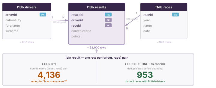
What COUNT(*) actually counts
When you join results to races, each result row stays attached to its race row. A race with twenty drivers produces twenty joined rows — one per driver. COUNT(*) then counts those twenty rows, not one race.
For British drivers, there are typically two to four British drivers on the grid in any given season. COUNT(*) adds one for each of them. Over seventy-plus years, that accumulates to 4,136 result rows — not 4,136 distinct races.
The correct query uses COUNT(DISTINCT raceid):
select d.nationality,
       count(distinct ra.raceid) as race_count
  from f1db.drivers d
  join f1db.results r  on r.driverid = d.driverid
  join f1db.races   ra on ra.raceid  = r.raceid
 group by d.nationality
 order by race_count desc
 limit 8;
 nationality │ race_count
═════════════╪════════════
 British     │        953
 French      │        835
 Italian     │        797
 Brazilian   │        791
 German      │        790
 Finnish     │        616
 Australian  │        606
 Austrian    │        559
(8 rows)
953 is the correct answer for British. There have been 953 championship races in which at least one British driver participated — not 4,136.
The wrong result (4,136) was off by a factor of 4.3. The error was invisible because the number was plausible in isolation.
What COUNT(*) is actually doing
SQL’s COUNT(*) is straightforward: it counts the rows in the relation it operates on. After a join, that relation is the Cartesian product filtered by the join conditions — one row per matching pair. If you joined results to races, you have one row per (driver, race) pair. COUNT(*) counts pairs.
To count distinct things after a join, name the thing:
count(distinct ra.raceid)    -- distinct races a driver appeared in
count(distinct d.driverid)   -- distinct drivers who appeared in a race
count(distinct r.constructorid) -- distinct constructors active in a season
The difference matters most when the join is one-to-many or many-to-many. In a strict one-to-one join, COUNT(*) and COUNT(DISTINCT pk) give the same answer — which is why AI-generated queries often pass superficial review.
The diagnostic question
After any join, ask: what does one row in this relation represent?
In results JOIN races, one row represents a (driver, race) pair.
If the question is “how many races?”, the answer is COUNT(DISTINCT raceid), not COUNT(*).
If the question is “how many starts?”, the answer is COUNT(*) — because that is exactly what you are counting.
Many questions that sound like “how many X?” are actually “how many distinct X?”, and AI tools default to COUNT(*) because it is simpler to write. Recognizing the join structure is the only way to know which one you need.
Making the overcounting visible
The two numbers — 4,136 and 953 — are related by exactly the average number of British drivers per race. You can make that relationship explicit:
with per_race as (
  select d.nationality,
         ra.raceid,
         count(*) as drivers_in_race
    from f1db.drivers d
    join f1db.results r  on r.driverid = d.driverid
    join f1db.races   ra on ra.raceid  = r.raceid
   group by d.nationality, ra.raceid
)
select nationality,
       count(*)                                                                     as races,
       round(avg(drivers_in_race), 1)                                              as avg,
       round(percentile_cont(0.5) within group (order by drivers_in_race)::numeric, 1) as median,
       round(percentile_cont(0.99) within group (order by drivers_in_race)::numeric, 1) as p99
  from per_race
 group by nationality
 order by races desc
 limit 10;
 nationality │ races │ avg │ median │ p99
═════════════╪═══════╪═════╪════════╪══════
 British     │   953 │ 4.3 │    4.0 │ 12.5
 French      │   835 │ 3.3 │    3.0 │  7.0
 Italian     │   797 │ 4.2 │    3.0 │ 14.0
 Brazilian   │   791 │ 2.5 │    2.0 │  4.0
 German      │   790 │ 2.7 │    2.0 │  6.0
 Finnish     │   616 │ 1.5 │    2.0 │  2.0
 Australian  │   606 │ 1.2 │    1.0 │  2.0
 Austrian    │   559 │ 1.2 │    1.0 │  3.0
 American    │   469 │ 2.7 │    2.0 │ 34.0
 Belgian     │   426 │ 1.3 │    1.0 │  3.0
(10 rows)
British: 953 races × 4.3 average drivers per race = 4,136. That is exactly the number the first query returned. COUNT(*) was not wrong about anything — it correctly counted 4,136 (driver, race) rows. The mistake was treating that count as an answer to “how many races?”
The p99 column tells an additional story. American drivers appear in 469 distinct races with a p99 of 34 drivers — a trace of the Indianapolis 500 era, when American fields were dominated by local entrants. Finnish drivers cluster tightly at median 2, p99 2: Finnish F1 participation was always a small, elite group. The shape of the distribution says something real about how each nationality has participated in the sport.
COUNT(DISTINCT raceid) opens the door to this kind of analysis. COUNT(*) closes it.